Alberta Clippers and Prairie Schooners

#2611 "Winter Tree Tunnel" 
20x16 inches oils gallery wrapped
40 centimetres of Singleton snow
after a Prairie Schooner

In the past few Science Stories, we have established how lee cyclogenesis is linked to conserving the spin of a figure skater. We briefly investigated how the temperatures of the equatorial Pacific Ocean influences the location of the jet stream and why there were more Alberta Clippers in a LaNiña year like 2022.  These storms are an essential part of the global balance. Weather results from an imbalance in one or all of the basic components of the energy cycle: heat, cold, water, electrical charge and there are certainly other forms of energy to juggle and try to distribute judiciously.

In advance of a low pressure area (a storm), warm and moist air is moved northward. In the wake of that low, cold and relatively dry air is moved southward. The pressure pattern that results is really a wave in the atmosphere … the downstream ridge is separated from the upstream trough by the storm and the next upstream ridge. Together the atmospheric wave which is the storm attempts to keep the earth in balance. The wavelength is from one ridge to the next. 

The impact of an atmospheric wave is related to its size - just like waves on the ocean. Winter weather can also have more impact than summer. Although severe summer convection can be extremely exciting and dangerous, the impacts on society and the economy are often more important with the winds, temperature and precipitation of “ordinary”, everyday winter weather. Such is the case with Alberta Clippers and this is where we have been headed all along. 

Genesis Stage of an Alberta Clipper

The impacts of Alberta clippers also vary with the size of the storm. The scale of an individual clipper varies with the strength of the jet stream crossing the Rockies, the size and intensity of the lee cyclogenesis and the temperature contrast across the frontal zone. There are other factors for sure but let’s keep this simple. We will even start with some history. 

The name “Alberta Clipper” was coined in the late 1960s by Rheinhart Harms, a meteorologist at the U.S. National Weather Service Office in Milwaukee, Wisconsin. Rheinhart witnessed the rapid speed of these snow storms as they crossed the Prairies. I undoubtedly heard the term when I entered the world of meteorology in the 1970s. It would take until the 1990s for that phrase to enter the scientific literature.

Alberta clippers are frequent winter forecast challenges and can occur every few days in rapid succession just as they did in February 2022. The first clue is to witness the jet stream crossing the Alberta Rockies nearly perpendicularly. A chinook arch is typical when those westerly winds charge down the lee slopes to dig the lee the trough. The chinook brings relatively warm weather approaching 10 °C even in the middle of winter. Lee cyclogenesis follows as the energy of the jet stream and the “figure skater” is transformed into a low pressure area and wave that then ripples along with the jet stream.

The clippers approach fast. Snowfall amounts with these systems tend to be small with only 3 to 8 cm being typical. The lack of moisture and short duration keep the accumulation well below the warning impact threshold of 15 cm per 12 hours. 

The wind and the wind chills can be more important for the typical clipper. Temperatures typically drop 15 to 20 Celsius degrees in just a few hours behind the clipper cold front. Blowing and drifting of even the small amounts of snow can make travel treacherous in whiteout conditions. These situations can approach warning criteria. 

Alberta Clipper crossing the Great Lakes

As the clipper cross the Great Lakes, the dynamics of the storm can change. When combined, the five great lakes represent a huge source of heat and moisture as well as lower friction. The inland seas also provide the opportunity for the generation of snowsqualls when those strong, cold Arctic winds blow over the open waters of the lakes. Snowsqualls bring significant snow accumulations onshore as well as extensive whiteout conditions  – that is another story that we call lake-effect snow. Suffice it to say that Alberta Clippers can take on a different and potentially dangerous character when they cross the Great Lakes to affect Ontario, Quebec and the north-eastern United States. 

I spent a large part of my meteorological career very concerned about how Alberta Clippers would influence my forecast regions. In the early 1990’s I was looking for a simple way to differentiate between the impact and the threat of each of these storms emerging every few days from the Rockies of Alberta. The larger the storm, the more probable that warning criteria would be breached and this could all be summarized by the speed of the clipper. 

I started using the phrase “Prairie Schooner” to describe these larger storms that would produce warning criteria weather. Clippers were built for speed but for me, schooners delivered the goods! Often, clippers were rebuilt into schooners as they crossed the “Great Lakes Aggregate” as we described the combined effects of those inland seas. As I recall, clippers would sail along at about 30 knots but schooners moved slower at only 20 knots. I kept careful histories of the track and speed of these storms emerging from Alberta. Any clipper that was slowing down to 20 knots was doing so for good meteorological reasons and I would get ready to hoist the warnings and rebrand that weather event as a Prairie Schooner. 

The science of the storm was all embedded in the speed of the system. Temperature contrast, precipitation rate and duration, latent heat … there is a long list that goes into determining the size of the storm. And size determines the wavelength which governs the speed. 

In 2005 my meteorological career took me to COMET (https://www.comet.ucar.edu/) in Boulder, Colorado. I recall that the acronym stands for something like “Cooperative Program for Operational Meteorology, Education and Training” but no one in that office even uses that anymore. Some of these Blogs were turned into Training Modules by the professional team of instructional designers, scientists, graphic artists, multimedia developers, and information technologists of COMET, UCAR and NOAA’s National Weather Service. After seven years in Boulder, I gradually retired during the course of the last decade – but not totally. 

The distinction between Alberta Clippers and Prairie Schooners has possibly been forgotten or perhaps I did not explain the concepts well enough. This Blog was intended to mend the sails on that ship – the concepts are simple, effective and fun at the same time. 

Next week we will explain why small Alberta Clippers are faster than Prairie Schooners. It will all make sense with the assistance of meteorologist Carl-Gustaf Arvid Rossby and our friend the figure skater as we conserve spin also known as angular momentum. 

Warmest regards and keep your paddle in the water, be safe,

Phil the Forecaster Chadwick

Lee Cyclogenesis

#2618 "Flurry of Saturday Afternoon Activity"
10x10 inches depicting the weather of
an Alberta Clipper, February 2022

I no longer look at the weather as closely as I did. I spend more time painting now. But these Blog exercises allow me to revisit the meteorology and maybe relearn it better. Being retired, I can take that time to really savour the science and the beauty of how nature works. My goal is to spread that joy of nature to others. Appreciation of the natural world is the first and most important step in its preservation. 

Knowing the weather requires knowing the wind. We have been aiming at understanding the wind for the past couple of months. 

To quickly recap, we explained how the pressure gradient, Coriolis and centrifugal forces create wind in the free atmosphere on the spinning Earth. We added in the force of friction to better understand how winds move near the surface. Finally we spent a couple of week’s figure skating and conserving spin while moving that wind over mountains. We arrived at a better appreciation of why there is a ridge of high pressure over and upstream from those mountains and a trough of low pressure downstream. And that leads us to the lee cyclogenesis of storms and some very important weather. 

Lee cyclogenesis is a very reliable forecast when strong winds cross the Rockies… nearly perpendicular. The storms that result are determined by where the jet stream crosses those mountains and are typically named by the location of the subsequent lee trough. You have most certainly heard of Alberta Clippers, Colorado, Texas and Gulf Storms. The meteorology behind every storm is unique so that these averages are just my generalizations. If you put five meteorologists in a room, you are likely to get six opinions. Mark Twain might have said that “all generalizations are false, including this one” but generalizations can be useful so let’s continue. 

You might be surprised to appreciate that our weather is shaped by what happens over the Pacific - the El Niño-Southern Oscillation (ENSO). The typical jet stream locations in La Niña years are the black line generalizations in these graphics. The preferred La Niña locations of the jet stream flows are in dark blue. 

In El Niño years, the mid latitude polar jet stream can be diverted by a large, warm and dry ridge of high pressure. This large ridge can spread mild winters temperatures all the way eastward to Ontario. The southern, subtropical or Pacific jet stream is directed more across the extreme southern US in the El Niño phase. The science behind ENSO is extremely interesting and important story too but best left for another day. 

El Niño-Southern Oscillation (ENSO) and
Jet Stream Location Generalizations

The average path of the jet stream is revealed 
from the temperature anomaly for the month.
 Remember to place
your left hand in the cold blue
and your right hand in the warm red
and you are looking
in the direction of the wind.  The 6th warmest 
February on record was actually cold 
over eastern North America. 

This past winter was characterized by the La Niña phase of the El Niño-Southern Oscillation (ENSO). The jet stream is variable in location but is typically centred over the mid latitudes from southern British Columbia and Alberta to Colorado. This should be no surprise given how many Alberta Clippers raced across the Prairies and the Great Lakes Basin this past winter. From my vantage in eastern Ontario, it was a refreshingly typical cold season full of cold, snow, ice and wind... and it is not over yet. 

You might also be surprised that this cold pattern over eastern North America is the direct result of Global warming. I have explained this process many times but not today. The climate is changing dramatically as a result of human activity. In the short term, eastern Ontario will be spared from the baking inferno to the south and west and also receive precipitation. This cold and snow of winter can be a good thing. 

The equatorial sea surface temperatures were below average across the eastern Pacific Ocean (La Niña) this past winter and the odds are 53% that this pattern will continue into the Northern Hemisphere summer ... but that is another story. Through my research in performance measurement, I discovered a pattern that supercellular convection (the kind that is responsible for almost all severe thunderstorm events) was favoured over pulse type thunderstorms during the La Niña phase of ENSO. There are very good meteorological reasons for this but I needed more time and data to be certain of those facts and that is another story as well. So many stories... so little time. 

Next week we can bring an end to winter with a revisit to Alberta Clippers and why they are so very important. 

Warmest regards and keep your paddle in the water, be safe,

Phil the Forecaster Chadwick

Revisiting Mountain Ranges and Conserving Spin

 

#2608 "Red Cedar Snow Load" 16x20 inches
This snow came from a storm that originated in a lee
trough on the eastern flanks of the Canadian Rockies

In "Mountains and Balancing Spin", I tried very hard to explain what happens to air flowing over a mountain barrier. Certainly last week’s description of the dynamical processes that occur when the jet stream crosses a mountain was a bit challenging.

As a Special March Break Version of Science Tuesday, let’s revisit that material in another way before we describe how the mountain ridge of high pressure and the downstream lee trough fundamentally influence our weather. Everyone learns differently but when the concepts get into the grey matter, you will enjoy them for life. 

Conservation of angular momentum is always important and forever working in the background whether you are a figure skater or air moving on the globe. Changes in the skater’s rate of spin seems like magic when the rapid twirl of an "upright spin" slows to the leisurely rotation of the "camel or Campbell". The slow spin does not look anything like the desert dromedary! Apparently the name arose because it sounded similar to an Australian skater  with the Campbell surname who was famous for performing the "camel"  spin - both names sound very much the same. 

The change in rotational speeds arises because angular momentum must be always conserved if there is no friction. A small girth cylinder will spin much quicker than when the cylinder is squashed and that mass spread further from the axis of rotation. As mentioned, the same experiment can be completed using exercise weights and an swivel chair but figure skaters are more entertaining. The physics is the same.

The total spin of an air parcel must also be conserved as it crosses a mountain. That total spin is comprised of the spin in the air and the location of that parcel on the spinning Earth - we can call that "planetary spin".

Crossing the mountain results in the cylinder being squashed on the upwind slope. The resulting slower "camel spin" is offset by a deflection of the air toward the pole and a higher planetary spin. The total spin is unchanged.

After crossing the summit, the air flowing down the lee slope converts the camel into the upright spin. The quicker spin is offset this time by a deflection toward the equator where there is lower planetary spin. Once again the total spin remains the same. 

Looking Down on a North-South Mountain Range in the Northern Hemisphere
and the path of the air as described in words above

The total spin of the air crossing the mountain means that the air is deflected toward the pole on the upwind slopes and toward the equator to the lee of the mountain. The path of the air is simply the wind. 

From "The Answer Really IS Blowing in the Wind", we know that the wind follows the pressure height contours. As a result, the height contours also follow the path of the air - the wind. And thus we have a ridge of high pressure over and upstream from the mountain and a trough of low pressure in the lee.

700 mb Pressure Contour Map 
Essentially the Height Above Sea Level 
where the pressure is 700 mb
Averaging around 10 thousand feet above sea level

Ridge over the Rockies and Lee Trough
of Lower Pressure

Following the pressure height contours on a weather map is like cattle paths tracing height contours on a topographical map. In the free atmosphere without friction, the winds generally follow the height contours. If your left hand points toward low heights and your right hand to higher heights, you must be looking in the direction of the gradient wind. 

That ridge of high pressure over the mountains of western North America and the trough of low pressure in the lee of the Rockies, means a lot for our weather. The Rockies don't move much so the forecast problem reduces to predicting when strong winds will blow roughly perpendicular to the mountain range. The lee troughs have favourite formation locations - western Wyoming and Colorado is one, southern Alberta is another!

Weather is not magic. It can be understood just like appreciating when angular momentum is conserved and figure skaters produce marvellous displays while conserving spin. Skating and the weather can be amazing but they are not magic.

The forces acting on air moving over the mountain reach a physical solution that creates a ridge of high pressure over and upstream and a trough in the lee of that barrier. Air impacting perpendicular to a mountain on a spinning Earth has to move according to the laws of physics and conserve angular momentum… spin. Any confusion that results from this explanation is purely my responsibility. 

Now what does that mean for the weather? Lots! But let's save that for next week. 

Warmest regards and keep your paddle in the water,

Phil the Forecaster Chadwick

Mountains and Balancing Spin

#0610 "Wild Life"
Big storms that bring lots of snow like this requires
looking at the mountains and spin... 

Last Science Tuesday in “Angular Momentum Spins Up the Winds of Climate”, we were all in a spin about the conserved nature of angular momentum and figure skaters. Lots of wonderful nature exists as a result of living on a globe spinning on an axis tilted toward a star. The sun is our source of all energy, past, present and future.

The total angular momentum of our figure skater is actually comprised of two parts. The dominant portion that we examined last week is the large and exciting component comprised of the rapidly rotating skater on the ice. The other portion that is always in the background, results from the location of the skating rink. If the rink is at the North Pole (the northern tip of the Earth’s axis of rotation), our skater and everyone else in that arena rotates once every day. That  rotation is fast considering that we are simply standing there doing nothing. Pointing the thumb of our Coriolis Hand upward means that our fingers are curled in the same sense as the cyclonic rotation. The meteorological convention is that cyclonic rotation is positive and in the same sense as the rotation of the Earth. 

To make things easier, we had also better point out that angular momentum has two aspects – the speed of rotation (spin) and the pointing direction of the rotation axis. At the North Pole the rotation axis of the skater is aligned with the rotation axis of the Earth. The cyclonic spin of the skater is augmented by the cyclonic spin of the Earth. 

If that skating rink is gradually shifted along any line of longitude from the North Pole toward the equator, the axis of rotation of the skater becomes less aligned with that of the Earth. At the equator the rotation axis of the skater is perpendicular to that of the Earth. Imagine a stationary skater looking eastward at the equator. The skater does not spin at all as the earth does its daily rotation. The ice rink has also melted.

The total angular momentum of the skater is the sum of these two components of spin and that total is conserved in the absence of friction. The component of angular momentum that results from the location of the rink is typically called “planetary angular momentum” by meteorologists as the Earth is doing all of the work. To keep things simpler and save a dozen letters on each repitition, let's just refer to the angular momentum as "spin" from now on and remember that it is conserved. 

Now let’s replace the skater with a cylinder of air of constant mass.  As noted in “Isentropic Surfaces - Science and Art Merges”, air follows isentropic surfaces for free with no exchange of energy. Spin must also be conserved for flows following constant energy surfaces in the absence of friction. 

In this thought experiment, we constrain the lid of the cylinder of air to follow a cold and higher isentropic surface while the bottom follows an isentropic surface near the ground. What happens when we move this cylinder with the westerly mid-latitudinal winds along a line of latitude? What then happens if we place a north to south mountain range in its path? North to south mountain ranges are actually quite common on the Earth but that is another story that makes nature and the weather so very interesting. 

The isentropic surface near the ground follows the west to east terrain profile closely.  The higher isentropic surface is a smoothed out version that spreads out the sharpness of the terrain features. As one would expect, the biggest impacts on the cylinder of air are felt over the mountain but there are significant implications both upstream and in the lee of the mountain.

Between 1 and 2 in the accompanying graphic, the upper isentropic surface has already started to feel the spread out effects of the mountain but not so much at the surface. The girth of the cylinder decreases thus increasing its spin like the figure skater pulling in her arms. To maintain a constant total spin, the parcel responds by diverting a bit to the south where lower values of planetary spin occur. 

At 2 when the bottom of the cylinder first reaches the mountain, the cylinder is rapidly scrunched into a squat can. This is like a skater very quickly loosing height and spreading that weight outwards far from the axis of rotation (like what happens in a “camel spin”). There is a big decrease in the cylinder spin and the cylinder itself must take a sharp turn to the north in order to gain higher planetary spin. The total spin is still constant. 

At the mountain peak (3), the bottom of the air cylinder starts to rapidly drop following the sharp terrain. The air cylinder is rapidly stretched and the girth decreases. The cylinder spin increases dramatically. The air cylinder takes a rapid detour to the south in order to reach the lower planetary spin values at lower latitudes. The total spin is still the same as what the cylinder had when it started. 

Once the cylinder reaches the plains at 4, the stretching is reversed and the cylinder girth increases. The vertical height of the cylinder starts to decrease again as the upper level isentropic surface starts to get far enough away from the influence of the mountain. The spin of the cylinder starts to decrease and the cylinder turns again to the north to offset that loss of cylinder spin with the increased planetary spin found at higher latitudes. 

The air cylinder overshoots the original latitude. A series of ridges and troughs that gradually decay in amplitude then form downstream from the mountain. 

The dashed line mapped on the accompanying graphic (mountain barrier at 3) is the path of the cylinder with respect to the Earth as it was described above in words. The direction of motion of this air cylinder is simply the wind. The implication is that the trajectories of these cylinders or parcels of air over time must also be pressure height contours that describe the geostrophic wind.  In “The Answer Really IS Blowing in the Wind”, the wind was found to follow the pressure height contours. The diversion of air parcels to conserve spin must also change the pressure patterns around the mountain. A ridge of high pressure is created over and upstream of the mountain, while a trough of low pressure is formed downstream in the lee of the mountain barrier. And all as a result of conserved spin on a spinning Earth. Wow. 

If we look at the change in pressure along the dashed line of latitude in the image above, we see this. A high pressure over and upstream from the mountain generates a pressure gradient force (PGF) pointing eastward toward the lee trough. This PGF blows on the mountain barrier and returns westerly momentum that was picked up by the atmosphere in the tropics back to the Earth. This poleward transport of westerly momentum from the tropics to the mid-latitudes keeps the total spin of the earth biosphere in balance. 

Next week will reveal what this means for the weather… it will be worth waiting for. My friend and professor from the University of Alberta, Dr Edward Lozowski had a careful look at this week's Blog and offered some invaluable suggestions making it both simpler and better. Thank you my friend!

Warmest regards and keep your paddle in the water,

Phil the Forecaster Chadwick

Angular Momentum Spins Up the Winds of Climate

#2068 "Mattawa Outward Bound" 24x48
Coriolis might have been deflecting our canoes to the right...
and I am pretty certain I saw vortices and deformation zones in the
current of the Mattawa... but angular momentum was preserved. 

Angular momentum is conserved in a closed system. Rotational energy is angular momentum that can be converted from one form to another but never lost - although we might not be able to get it back either.  

w= angular speed or rotation

The figure skater is everyone’s perfect analogy for angular momentum, although the skater is not a perfect closed system. The sound of the skate is a loss of rotational energy. Friction with the air and ice is another energy loss. The rotational speed is controlled by the "moment of the mass distribution" but with time, even the best skater will spin down to a standstill. The figure skater can control their rate of rotation. If they extend their arms and legs outward from the axis of rotation, their moment of mass distribution increases and they spin slower. Skaters spin faster by pulling their body inward to their rotational axis thus minimizing their moment of mass distribution. In all cases, their angular momentum is unchanged although they gradually spin down as that energy is lost.  The conservation of angular momentum through the re-distribution of mass can also be also studied using a swivel chair and exercise weights but the artistic impression points will not be nearly as impressive. 

Earth and the Moon as
seen from Mars orbit

Consider the earth. You might think that the spherical blue marble spinning in the vacuum of space is a perfectly rigid and closed system.  The earth might be close to that ideal but consider that scientists study the variable length of day (LOD). The "LOD" has actually increased over the 4.54 billion year history of the Earth due to tidal effects and the dissipation of angular momentum. The earth is spinning down. 

The Moon at about 1/81 the mass of Earth, is slowing the Earth's rotation. Days get about 2 milliseconds longer every 100 years. The moon has already stopped spinning and the tidal locking process will theoretically do the same to the Earth in 50 billion years. Weather would be very different on a stationary planet and your Coriolis hand will no longer work very well.  

Length of Day Deviations since 1965

The LOD also fluctuates on shorter times scales.  These miniscule variations have periods that range from a few weeks to years.

Outer Mantle - Liquid Outer Core- Solid Inner Core

The total angular momentum of Earth as a whole system must be constant. The relative movements and mass redistribution of Earth's core, mantle, crust, oceans, atmosphere, and cryosphere (cryosphere is the frozen water part of the Earth system) will result in variations in the spin (LOD) just  like the figure skater. A change of the angular momentum in one region must necessarily be balanced by angular momentum changes in the other regions.

The mass of the earth is far from evenly distributed. The continental plates are shifting. The polar ice caps are calving and breaking apart. Glaciers are melting. Mass is slowly being redistributed. The 'decade fluctuations' of Earth's rotation rate and LOD are thought to result from these fluctuations.

The LOD also varies significantly over time scales down to weeks.  We can blame these on the weather. Consider the water cycle for instance. Water evapourates into water vapour and rises, increasing the moment of that mass distribution. Precipitation falls to the ground and the moment of mass distribution decreases again. Storms can move this precipitation toward the poles and these movements also decrease the moment of mass distribution on the spherical globe. The increasing temperatures of climate change allow about 7 percent more water vapour to be held in the atmosphere for every degree Celsius of increase. The moment of inertia for that increased amount of water vapour higher in the atmosphere would be expected to slow down the Earth's spin - a longer LOD results. 

Observational evidence shows that there is no significant time delay between the change of  the atmospheric angular momentum and the corresponding impact on the LOD. The atmosphere and solid Earth are strongly coupled due to surface friction with a time constant of only about 7 days which is the spin-down time of the Ekman layer. We met Vagn Walfrid Ekman (1874 – 1954) in "Meteorology Meets Oceanography". This spin-down time is how long it takes to transfer atmospheric axial angular momentum to the Earth's surface and vice versa.

We need only consider the component of the zonal wind  (along the lines of latitude) at the ground to consider the transfer of axial angular momentum between the Earth and atmosphere. Textbooks  describe the rigid rotation of the atmosphere with the zonal wind with a speed of "u" at the equator relative to the ground. Super-rotation of the rigid atmosphere is when u > 0 and the rigid atmosphere is  rotating faster than the earth. If  u < 0 indicates then the rigid atmosphere is rotating slower than the Earth and "retrograding". The meridional wind (along the lines of longitude) and the vertical wind move the atmospheric angular momentum around the globe but these must balance out with time - due to the weather which is next week's Science Tuesday. 

Climatic Global Wind Patterns 

Surface friction allows the atmosphere to gain angular momentum from the Earth in the case of the atmospheric retrograde rotation or release it to Earth in the case of super-rotation. In the climatic average, the ground level zonal wind-component responsible for rigid rotation must be zero. This fact can explain the global wind patterns. The prevailing winds in the tropics and over the poles are easterly trade winds. Between 30 and 60 degrees the winds are westerly.  The atmosphere gains angular momentum from the Earth at low and high latitudes and repays that same amount back to the mid latitudes. Nature likes a balance. 

These musings and the posts of the last several weeks have been intended to ponder how complex yet beautiful the moving atmosphere can be - wind. We can now better understand the winds of weather from first principles - pressure gradient force, Coriolis force, centrifugal force, friction and finally the winds of climate (angular momentum balances). Some brilliant scientists were curious and discovered these natural wonders out over the last couple of centuries. It is important to remember these natural wonders and the scientists as well. 

The LOD might vary by a fraction of a millisecond as the atmospheric angular momentum is moved around the globe but that is not going to impact any forecast. Meteorologists simply do not have the time to worry about the LOD or to think of the angular momentum of the Earth and its components in order to forecast the wind. But next week we will look how these concepts might be used to better understand storms and the weather - know the wind; know the weather. Please stay tuned... 

Warmest regards and keep your paddle in the water,

Phil the Forecaster Chadwick

Meteorology Meets Oceanography

#0135 "Tiger on the Prowl"

Energy is neither created or destroyed… but energy is often converted from one form into another. In "Adding Friction to the Wind Balance" I described how friction with the earth in the planetary boundary layer (PBL) would always turn the gradient wind (see "Another Look at the Wind") toward lower pressure. Your Coriolis arm would turn toward lower pressure with increased friction and if you kept your thumb pointed in the direction of the pressure gradient force, the angle between your thumb and fingers would get smaller with increased friction. 

Summary Explanation of the Gradient Wind,
Friction and your Coriolis Arm

Vagn Walfrid Ekman (1874 – March 1954)

But I did not mention Vagn Walfrid Ekman! Yet... Dr Ekman (1874-1954) was a  brilliant Swedish oceanographer as well as a musician. Art and science are once again intertwined. The Norwegian explorer Fridtjof Nansen was the science officer on the voyage of the Fram 
1893–1896 which was tasked to reach the geographical North Pole by harnessing the natural east–west current of the Arctic Ocean. During the expedition, Nansen observed that icebergs tended to drift not in the direction of the prevailing wind but at an angle of 20 to 40 degrees to the right. Hmmm. Bjerknes invited Ekman, still a student, to investigate the problem. Vilhelm Bjerknes you might recall, could be called the father of modern meteorology as he formulated the primitive equations that we use in  meteorology and numerical weather prediction. Vilhelm and his son Jacob figure prominently in "Weather Dances" where I discus their Norwegian cyclone model and the military terms used therein since they did much of the work with the backdrop of World War One. 

Anyway, in 1905, Ekman published his theory of the Ekman spiral. His theory explains the  balance between frictional effects in the ocean and the Coriolis force which exists because we live on an non-inertial frame of reference - the spinning planet. 

The science of meteorology and oceanography were incredibly intertwined more than a hundred years ago. 

Now back to the energy conversions to drive this point home. The wind energy of the free atmosphere is transformed by friction with the earth’s surface into angular momentum of the earths rotation (more on this in another blog). In addition, as the wind approaches the rough surface, your wind balanced Coriolis arm turns toward lower pressure and the wind speed decreases with that energy shoving the earth along. This is the Ekman spiral in the atmosphere as pictured above using my waving hand and arm. 

Oceanographic Ekman Spiral
where
1 is the friction PBL wind,
2 is the force from above,
3 is the direction of the resultant current
 (vector addition) and
4 is the Coriolis force 

When the atmospheric winds lower to the surface of the ocean, simply another fluid, that energy of wind motion is transferred to the water. The frictional driven water current is deflected by the Coriolis force - to the right in the northern hemisphere.  There is a net current to the right of the PBL wind. Along coasts, the net loss of surface water can  result in a secondary upwelling current. These coastal upwelling Ekman driven current explains the famous fisheries around the globe.  

The water brought to the surface from the depths is typically  rich in nutrients that support the coastal ecosystems. Declining oxygen with climate change is starting to counter these benefits. 

The energy of the atmospheric wind can drive the energy of the oceanographic Ekman spiral which in turn (so to speak) drives the coastal upwelling which encourages the fishery and feeds nations. Nothing is lost and all is sustainable IF this energy and these resources are managed wisely. 

Ekman driven Upwelling

Everything is connected...

Oceanography and meteorology are sciences of fluids on a spinning globe. Both are vitally important to the welfare of the planet and the creatures that share this garden of Eden. I have been a life long member and supporter of the Canadian Meteorological and Oceanographic Society. We are all in this together… air, water and sometimes even rock are fluids. Maybe we should add volcanology to the society of fluid sciences as well!

Warmest regards and keep your paddle in the water,

Phil the Forecaster Chadwick

Applying the Gradient Wind Balance... To Shovel or Not to Shovel... that is the Question

0519 "Homestead -West Wind"
Home and Watershed Farm in 1993

Happily, most of my career with Environment Canada spanned what I think of as the Golden Age of Meteorology – before technology took over. 

Map Analysis 1977

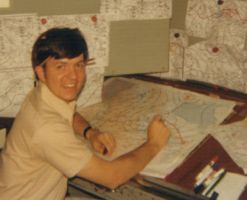
The forecast cycle was still a largely human exercise in the 1970’s. There was still so very much to study and humans learn by doing. The first step in every shift was to do a thorough weather analysis. I drew isobars on coloured maps with a terrain background. I had a plastic pocket protector full of coloured pencils and markers. The data had been hand plotted by an expert technician. The surface chart was a work of both art and science upon completion. The patterns revealed the current weather situation and the “concern of the day”. The team would concentrate on predicting the most important weather elements for the coming days. Life was very good, fun and full of challenges.

Some of the fruit from that Golden Age of Meteorology has been the remarkable numerical simulations of the atmosphere of today. The Numerical Weather Prediction (NWP) ingests far more data and completes billions of calculations beyond what humans can do. The essential super computers produce remarkably accurate forecasts that span space and time around the Globe. Meteorologists use these tools to aid clients in the increasingly weather sensitive society. But it is still important that humans understand the nature of weather and that leads back to these posts. 

The past few Blogs described how to interpret those isobars on the surface map and the height contours on the upper air charts. 

We started with the Geostrophic Wind Balance and then added in the centrifugal force to achieve the Gradient Wind Balance. See "The Answer Really IS Blowing in the Wind" and "Another Look at the Wind". Finally we added in friction to understand what happens to the wind in the planetary boundary level (PBL) where we all live. See "Adding Friction to the Wind Balance". After those Blogs, we have a basic understanding of the wind. 

Hand analyses are generally a thing of the past. The computer generated surface pattern from this past Saturday can still reveal what one needs to know. Blowing and drifting snow will restrict transportation and close schools as effectively as a general snowfall. To forecast those events can be complicated as it depends largely on the characteristics of the snow surface. The wind is the key factor though and those last three posts has gotten us to the point to answer those questions. 

The geostrophic wind based on the extremely tight spacing of those isobars alone, would be an under-estimate of the real gradient wind. The isobars over the lower Great Lakes are nearly straight if not curved anticyclonically. 

The observed winds for the same time as the surface chart show winds blowing on average of 45 degrees across the isobars toward lower pressure - the influence of friction. 

850 mb Height Contour Chart for about the same time.
 Note that the winds at about 5000 feet above the surface
away from friction, closely follow the height contours.

The important forecast was that Saturday was going to be a very blustery day with south to southwest, gusty winds. For me that meant that I would not bother to shovel the lane or sidewalk as the snow would just drift back into place. I painted in the Singleton Studio instead. 

Now we know the wind... and that  information can guide us in our decisions. 

Warmest regards and keep your paddle in the water,

Phil the Forecaster Chadwick

Adding Friction to the Wind Balance

 

#0839 "Cold Air Mass Cumulus"

There are four forces required to really understand the wind. 

• The pressure gradient force (PGF) varies with the contrast in pressure and points toward low pressure. 
• The Coriolis force defects moving parcels to the right (Northern Hemisphere); varies with the speed. 
• The Centrifugal force varies with the curvature and always points toward the centre of that curvature. The Centrifugal force influences the relative strength of the gradient and geostrophic balances. 
• Friction turns the wind to lower pressure… the more friction… the more turning. 

The PGF, Coriolis and Centrifugal forces determine the wind in the free atmosphere. Friction is important in the Planetary Boundary Layer (PBL) but all of the forces are required to understand the wind near the earth's surface.  

The Wind Balance of Forces including Friction

"Another Look at the Wind" explained how to use your Coriolis arm to understand the wind in the free atmosphere. We can use that same approach to understand the influence of friction in the PBL. Friction simply slows the air down. A rough surface like a forest is more effective than a lake in slowing the wind down. Using your arms and body to approximate the balance of forces to create winds is another reason why weather is a ballet.. a dance and not a battle.

Consider your Coriolis Arm that is attached to your Coriolis Hand. Align your arm with the gradient wind at the top of the PBL. Hold your Coriolis Hand outward with your fingers pointing in the direction of the gradient wind, your palm facing down and your thumb stretched at 90 degrees. Your thumb must point in the direction of the pressure gradient force (PGF) at all times. As you descend toward the earth's surface (in your mind), you start to encounter friction. The wind slows down but wants to stay in balance. The wind tries to keep blowing as fast as it did by turning to flow more toward the low pressure - down the pressure mountain. Your Coriolis arm will turn toward the lower pressure but keep your thumb pointing in the same direction that it was at the start - the direction of the PGF.  The effects of friction is approximated by the angle that your thumb makes with the rest of you Coriolis arm and fingers.

Your Coriolis Arm Can Illustrate 
the Impacts of Friction Too

In the homemade graphic, the gradient wind in the free atmosphere is in the top left. As one descends toward the ground, the Coriolis arm gets progressively obscured.. maybe it was a foggy day? The Coriolis arm on the lower right is at the ground level where we all live. 

Now we know the wind... 

Warmest regards and keep your paddle in the water,

Phil the Forecaster Chadwick

Another Look at the Wind

#2009 "Algonquin Rock Lake Turbulent Sunrise"
Looking back at this plein air painting, I see
that I painted my Coriolis hand into the
cold advection, turbulent stratocumulus. 

The geostrophic and gradient wind balance equations can be a challenge even for meteorologists. The fundamental forces that move the air around the Globe are not something that we think about every day. There is no time during any shift to go back to first principles when preparing a forecast for the next week for large areas of Canada. 

To be clear, what I am attempting to do in these Art and Science Blogs, is explain nature in a way so that even the most challenging concepts are understandable. It is a task I have set for myself and I link the ideas with phenomena that I observe in my artwork. Science should make sense and if I can’t explain something, then I must not really understand it well enough. Being naturally curious can be a full-time occupation - even when retired I need to brush up on the science and learn it better. 

I rely on visual aids when explaining things. Many of these explanations, especially meteorological ones, are hand-waving exercises. I do not go anywhere without my Coriolis Hand! The Coriolis Hand can be used to explain much about living on a rotating planet. 

Gaspard-Gustave de Coriolis of Paris (1792-1843) was an engineer and mathematician who first described motions on a rotating body deflected by an apparent force that now bears his name. If you place your Coriolis hand palm down and point your thumb in the direction of the motion, the moving substance will be deflected in the direction of your fingers. Your right hand is your Coriolis Hand in the Northern Hemisphere while south of the equator, it is your left hand. 

We can also use the Coriolis Arm which is attached to your Coriolis Hand, to explain the geostrophic and gradient wind balances detailed in the last Science Tuesday. I keep trying to elucidate things in different ways until the concepts connect. Everyone learns in their own unique way. 

The Geostrophic and Gradient Wind Balance Graphics

Instead of analysing the vector diagrams like we did last week, align your Coriolis Arm with the gradient wind at the top of the planetary boundary layer (PBL) - where there is no friction. Hold your Coriolis Hand outward with your fingers pointing in the direction of the gradient wind, your palm facing down. If you stretch your Coriolis thumb at 90 degrees to your fingers, your thumb must point toward lower pressure and in the direction of the pressure gradient force (PGF).  The Coriolis force deflects every moving thing to the right in the Northern Hemisphere. The centrifugal force always points way from the centre of curvature. 

The following graphic summarizes these three forces - pressure, Coriolis and centrifugal using your own Coriolis Arm. It also explains that due to the centrifugal force, the gradient wind is weaker than the geostrophic wind balance in a trough but stronger in a ridge.  My Coriolis arm only bends cyclonically when I am relaxed and one would expect the gradient wind in a trough to be more calm as well. 

Understanding the Wind Using you Coriolis Arm
View looking down from space

You can use your Coriolis Arm in reverse as well. Point your Coriolis fingers in the direction of an observed wind revealed by gravity waves, swells or Langmuir Streaks. Your stretched thumb must point toward lower pressure. If the wind is strong, the pressure gradient is also steep. All of these facts can tell you something about the weather. 

Next Science Tuesday we will add in the fourth important force of friction so that we might better understand the wind in the planetary boundary level as well. Bring your Coriolis arm too. 

Warmest regards and keep your paddle in the water,

Phil the Forecaster Chadwick