Wednesday, October 19, 2022

Tom Thomson Was A Weatherman - Summary As of Now

Thomas John Thomson (born 5 August 1877 in Claremont, ON;
died 8 July 1917, almost 40 years old )  circa 1905–10.                 
I started doing presentations about the art and science of Tom Thomson in the mid-1980s. I did not keep count, but the number of presentations certainly numbers in the hundreds. This mountain of material has grown into a book that is now being blogged a bit at a time. 

Thoreau MacDonald (1901-1989), the son of JEH MacDonald of the Group of Seven, was also a friend of Tom, and he wrote:

Thomson’s work would be a fine study for some competent critic, but anyone attempting it should be familiar, not only with every phase of his work but with the country too, lakes, rivers, weather; have them in his bones …

I prefer to be positive... being critical is not my style, but my natural science background brings fresh information to the Tom Thomson catalogue raisonnĂ©. This project will take some years to complete, but I am in no rush. 

In the draft of my "Tom Thomson Was A Weatherman" book, I included several chapters describing the meteorology and natural science employed to better understand his art. This information has already been written in "The Art and Science of Phil the Forecaster" blogs, which I have been compiling for many years. If you should encounter a term or concept that I do not adequately explain within the context of a particular Thomson work, a search of this site will certainly yield the answers. I will typically include linked references to the required background information with each painting. 

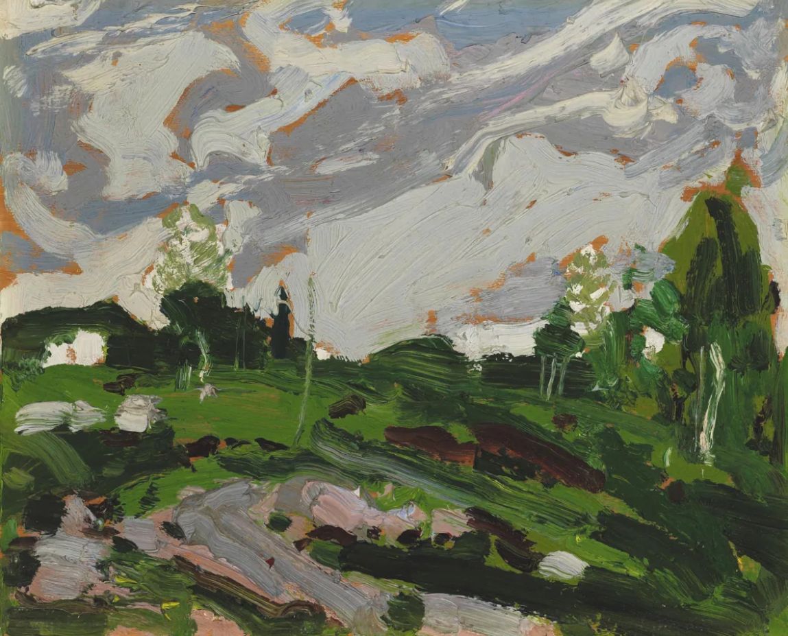
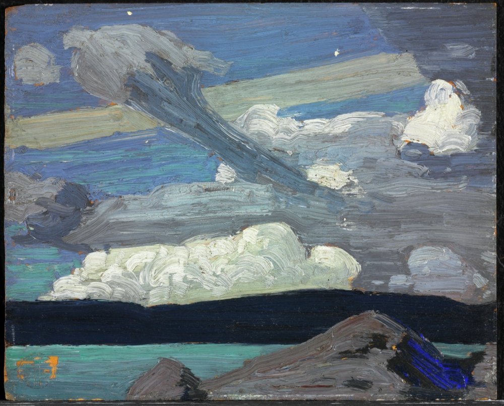
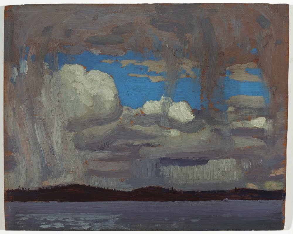
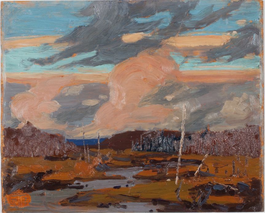
The following is a list of the Blog entries to date, accompanied by a representative image and a linked title to the Blog. Some paintings require more than one blog post to fully explain. Tom accurately painted the truth of what he saw. 

Arthur Lismer, his friend and Group of Seven member, described Thomson as someone who "sought the wilderness, never seeking to tame it, but only to draw from it, its magic of tangle and season." That wilderness put the "wild" into his art. 

Blodwen Davies included in the 1967 publication "Tom Thomson: The Story of a Man Who Looked for Beauty and for Truth In The Wilderness" that  Tom Thomson had remarked: "Someday they will know what I mean." Hopefully, that day has arrived.

Note: Miss Blodwen Davies's passed in 1966, but she had previously sought help from Group of Seven artist A. Y. Jackson, who had written the Foreword to the first self-published version in 1935. That first printing was limited to 100 copies, and the 1967 republished version of that scarce book is available to a larger audience. 

Thank you for your interest. These posts have been a lifetime in coming. 

Tom Thomson Was A Weatherman


Tom’s Tornado!


Tom’s Tornado Two - Some Science

Tom’s Tornado Three - Some Art


Tom's Summer Clouds


Thunderhead: Pink Cloud over a Lake - Summer 1916


Lightning, Canoe Lake: Summer 1915


Tom Thomson’s Last Weather Observation


Updated May 2024


Tom Thomson's "A Northern Lake" Was the Belt of Venus Sunrise
Tom Thomson's Black Spruce Autumn 1915 observation of a cold frontal passage
Tom Thomson's "First Snow in Autumn", Fall 1916 - Light and fluffy snowsquall snow laden on drooping balsam fir branches


Tom Thomson's Approaching Snowstorm - actually a snowsquall as contrasted with a synoptic scale winter storm.
Tom Thomson's After the Sleet Storm, 1916 - published 25 years after the 1998 Ice Storm and it brings back many personal memories.
Tom Thomson's Burnt Land at Sunset - the dynamics of the weather was Tom's inspiration. 


Tom Thomson's Afternoon: Algonquin Park, 1915 Studio Work in The Shack - Tom painted this in late November 1914 and one of his last works in the Studio Building before heading to the Shack. 

Tom Thomson's The Morning Cloud, 1913 Plein air sketch from the autumn of 1913. What an unusual cloud!

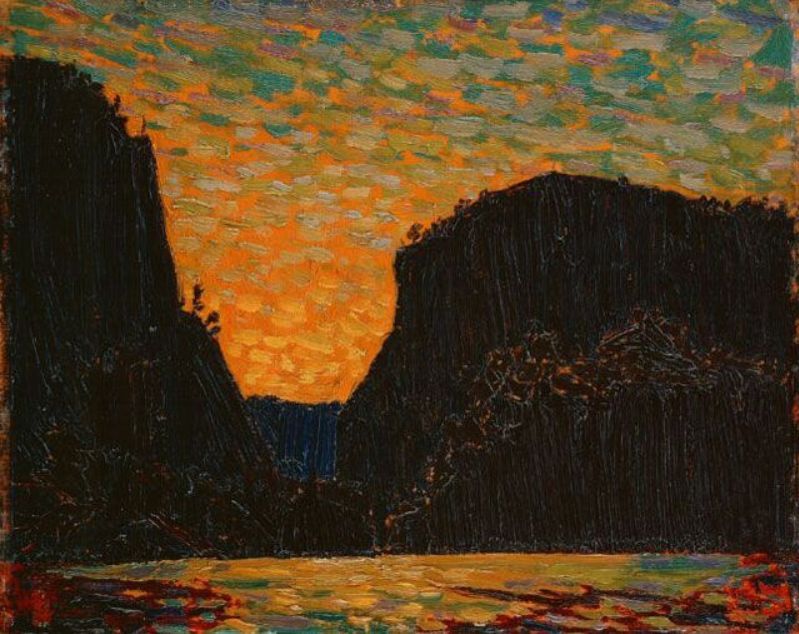
Tom Thomson's Petawawa Gorges Night 1916. The "fallout" from Creative Scene Investigation requires that "Petawawa Gorges, Night" along with the alternate titles "Sunset behind Cliff" and the "The Coming of the Night" need to be revised. The reality is that Thomson was a morning person and this painting was certainly a sunrise observation of light and shapes.


Islands, Canoe Lake, 1916. Some interesting meteorology and history. Tom Thomson spent some time at Canoe Lake in October 1916 after spending the summer being a forest fire ranger at Achray on Grand Lake. 

Landscape with Snow, 1916. Even more interesting meteorology and history. The flip side of Tom Thomson's “Rising Mist - Heavy Skies” Autumn 1916

Smoke Lake - Summer 1915. This is another of Thomson's double-sided panels and there is a story of weather and confusion behind it. 
The flip side of Northern Lights 1915.

Northern Lights 1915. The flip side of Smoke Lake - Summer 1915. Tom observed and recorded space weather as well. 

Path Behind Mowat Lodge, Spring 1917, The gift to Daphne Crombie includes a lot of interesting science as well. 
Canoe Lake Spring, 1917 - an afternoon sketch with the centre of the low-pressure area nearby turns into much more with the assistance of Roy MacGregor
Moonlight Over Canoe Lake 1916 A tremendous amount of science in this plein air panel...
Sunset Spring 1916 ... the view may not be what you think it is! 
Spring Sunset, Algonquin Park Spring 1916 also holds some surprises... this story was never told.
The Marsh, Early Spring 1916 - a challenge to place the location but not in the weather.


Sunset, Summer 1915. There is a lot of science in this painting and it was a spring sunrise (not sunset) painted around May 24th, 1915...

Sunset Sky, Summer 1915 was indeed a sunset but was observed in the spring.  
Sunset Sky, Spring 1915 was a spring painting but was actually a sunrise. This post has been years in the making and I have never included it in a “Tom Thomson was a Weatherman “ presentation. The last two posts lead to this one - a trio if not a quartet of skyscapes within a single event. 


Morning, Algonquin Park, Spring 1915. It was a dark and stormy morning at Canoe Lake that spring morning in 1915 when a cold front was crossing Mowat.
Ragged Pine, Spring 1916. Actually a black spruce but that is only the tip of the true story. 

Rocky Shore and Sky Summer 1915  The foreground was the devasted shore of Canoe Lake left behind by the forest industry.. lost habitats. The sky was full of interesting science!


Hot Summer Moonlight Summer 1915. Actually, a view overlooking Grand Lake from Achray possibly at 9 pm on May 11th, 1916... The waxing quarter moon spread the glow over the choppy waters of Grand Lake while a spring storm approached. And the story was recorded in Tom's brushstrokes. 

Sunset by Lake Alternate title: Sunset Summer 1915 Quite the back story behind this painting... 
Blue Clouds, Wooded Hills, and Marshes Summer 1915. Science Tuesday shines a new light on this painting... perhaps from 1916. 
Stormy Sky Summer 1915. Actually a split cold front mid-morning in spring. 
Fire-Swept Hills Summer or Fall 1915. Long-range Forecast: Continuing hot and dry for the rest of the 21st "Century of Fire". 


Ragged Lake Alternate titles: Northern Lake; Ragged Creek Fall 1915
Autumn Clouds Fall 1915 Dynamic cloud shaped by the wind bathed in the light of sunset tell an intriguing story of science and the weather.
Evening Cloud Alternate titles: Evening Clouds; Storm Cloud; Storm Clouds Fall 1915 Hers is the real story... cumulus congestus at a cold frontal passage wearing the Belt of Venus...

Artist's Camp, Canoe Lake, Algonquin Park Alternate title: Night Camp Fall 1915. There is a very interesting story behind the white "balloon silk", state-of-the-art tent. 
Tea Lake Dam Fall 1915 certainly painted in the spring with logs going to market - probably 1916. 
Moonlight Fall 1915 Actually painted in the spring of 1916... on the evening of April 18th about 18 hours before Ragged Pine, Spring 1916.
Abandoned Logs Fall 1915 Those logs were not abandoned in the spring of 1916 when Tom observed the log drive along Carcajou Creek. The tall pile of logs was a landing piled high by the hard-working lumbermen. 
Sketch for "The Drive" Fall 1916 After painting Abandoned Logs Tom probably strolled 100 metres along the western bank of Carcajou Creek to were the lumbermen were actively guiding logs through the sluiceway of the dam on the May morning in 1916. 
Sandbank with Logs, Summer or fall 1916  There is actually quite an interesting story behind this tangle of timbers... 
Bateaux Summer 1916 Actually Pointers and there is quite a story to be told. 


Yellow Sunset, Spring or Summer 1916 There are two sides to this very interesting story!


View from the Top of a Hill 1916. This is the flip side of "Yellow Sunset".  Together they tell quite a story. 

Aura Lee Lake Spring 1916. Aura Lee Lake which is now known as Laurel Lake was definitely not an arduous canoe trip downstream from Little Cauchon Lake where Tom and his friends were fishing and painting up a storm!
Early Spring in Cauchon Lake, Spring 1916. It was a challenge to locate the correct rocky face... still looking.
Algonquin Park, Spring 1916. There is a lot of science in this small panel... and we can even guess where Thomson was sitting. 
Birches, 1916 The sky was the real star of this painting.
The Lake, Bright Day, Fall 1916 The clouds tell the story. 

Spring Break-up, 1916 The underlying story is of a clear-cut forest with nothing to hold back the spring floods. The cracks in the shoreline ice hold those clues.
Portage, Ragged Lake Spring 1915 This is a story of icy swirls. Tea-stained ice pans swirling in the turbulent waters of the outflow from Ragged Lake during the spring flood.
Red Pines, Little Cauchon Lake, Algonquin Park, Spring 1916 The story can be discovered by strolling behind the Red Pines to take a closer look at the sky. 
The Sketch for the Jack Pine 1916. Imagine a solitary tree exposed on the rocky shore of a northern lake facing the elements alone. Simply staying alive was a victory. Thomson captured that iconic message in oils. "The Jack Pine" has become the metaphoric touchstone of the Canadian experience. Like the seeds of a torched Jack Pine, Thomson's art could only be sown after his death to inspire the next generation of artists. 
Little Cauchon Lake, Spring 1916 A story from the fishing trip of late April 1916. TT-134
Spring Foliage on the Muskoka River The tale of Thomson's Spring Foliage evolves into the story of three paintings completed on an early summer afternoon... TT-135


Tom Thomson's "Smoke Lake" 1912. The story of a multicellular thunderstorm painted from Molly's Island on Smoke Lake looking southward.  TT-199


Tom Thomson's "The Hill in Autumn" 1914. My first diagnosis of "The Hill in Autumn" really troubled me! Some subtle inconsistencies bothered me enough that the story did not get published in the first go-round. Tom painted the tilted vortices of mares' tails in the azure skies - they looked like birds.  


Tom Thomson's "Sunset and Shore", 1916. TT-Post 113. A painting, probably no one has seen before, from Dr. MacCallum's bequest to the National Gallery. The location and weather can be exactly determined and will follow upon completion. 


The Waterfall TT-Post 145
Pine Cleft Rocks Spring 1916 TT-Post 136
Little Cauchon Lake, Spring 1916 TT-Post 137
Landscape, Sunset Spring 1916 TT-Post 138
Tamarack Swamp Fall 1916 TT-Post 139
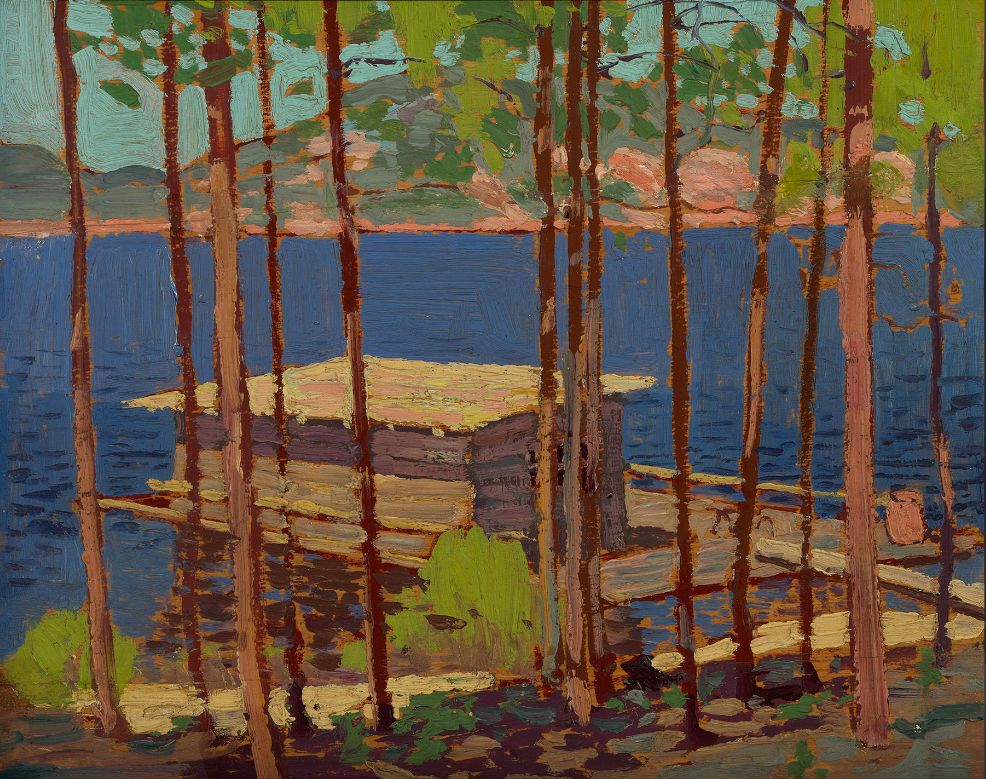
Boathouse, Summer 1916 TT-Post 140
The Dead Pine, Fall 1916 TT-Post 141

Autumn, Petawawa, Fall 1916 (1916.94) TT-Post 142


Algonquin Park Vista, Fall 1916 (1916.101) TT-Post 143


Spring Lake, Fall 1916 (1916.117) TT-Post 144


Pine Tree, Summer 1916 (1916.84) TT-Post 146


Phantom Tent, Fall 1915 TT-Post 90
Tamaracks Alternate titles: Purple Distance; Yellow Trees Fall 1915 TT-Post 91
Tamarack Swamp Alternate title: Tamarack Fall 1915 TT-Post 92
Round Lake, Mud Bay Alternate title: Geese, Round Lake, Mud Bay Fall 1915 TT-Post 93
November Day Alternate title: A November Day Fall 1915 TT-Post 94
Sunset, Canoe Lake Alternate title: Canoe Lake Fall 1915 TT-Post 95
Northern Lake Alternate title: Northern Lake, Spring Summer 1916 TT-Post 96
Poplars by a Lake Alternate title: Lake Through Trees Summer or fall 1916 TT-Post 97
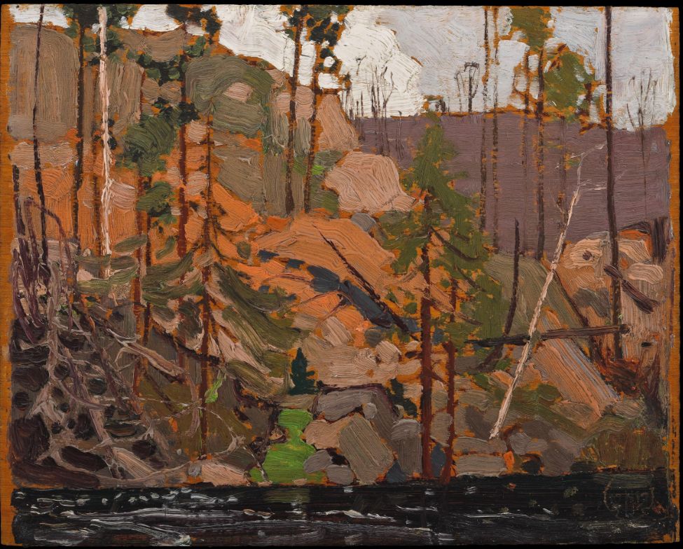
Petawawa Gorges Alternate titles: Cliff Landscape; Storm Over River Fall 1916 TT-Post 98
View from a Height, Algonquin Park Fall 1916 TT-Post 100


TT-Post 101
Somber Day Fall 1916 TT-Post 102

Ragged Pine Fall 1916 TT-Post 103
Birch by a Lake, with Big Cloud Alternate titles: Birch by a Lake; Birches; Clouds over a Lake Fall 1916 TT-Post 104
Autumn, Algonquin Park 1916 TT-Post 105
Lake in Autumn Alternate titles: Late Afternoon?; Swamp in Fall? Fall 1916 TT-Post 106
Canoe Lake, Algonquin Park Fall 1916 TT-Post 107
Pink Clouds Fall 1916 TT-Post 108
Wild Geese: Sketch for "Chill November" Alternate titles: First Snow Ducks; Sketch for "Chill November" Fall 1916 TT-Post 109
Sunset, Canoe Lake Fall 1916 TT-Post 110


TT-Post 111


The Pointers, Winter 1916–17 (1916-1917.13) TT-Post 112


The following final posts describe how several paintings might be connected in time and space.


Tom Thomson and the 1917 May Two-Four Weekend (coming)

The ability of nature to inspire and heal can be magical. The preceding articles were never intended to teach the incredible complexities of physics or meteorology. The goal was simply to encourage the reader to look at the natural world from a fresh perspective - to appreciate the magic of nature and perhaps become a "weather walker" and a protector of the environment. 

Tom was inspired by the supernatural that he witnessed through his brief forty years. That world is being threatened by unsustainable consumption, which is the source of all environmental issues. The reader inspired by Tom's art and nature might be moved to take action for future generations as we careen through the Sixth Mass Extinction and  Earth's Loss of Biodiversity. That was the other goal of this effort disguised as art history. Art and science can be compatible. 

Of course, you may simply wish to enjoy the art of Tom Thomson and that is absolutely fine as well - even encouraged! As Claude Monet said: “Everyone discusses my art and pretends to understand, as if it were necessary to understand, when it is simply necessary to love.”

I always left the last word for Tom Thomson at the end of every "Tom Thomson Was A Weatherman
presentation. On Saturday, July 7th, 1917, the day before he died, Tom wrote to his patron Dr. James MacCallum: "Will send my winter sketches down in a day or two and have every intention of making some more..." Tom was not finished with his artistic journey! Neither am I!

Tom Thomson May 1917 at the campsite firepit. The last picture of Tom that I am aware of...

There are many more articles to come but it takes time to translate the "Tom Thomson Was A Weatherman" book into blogs .. and I still need to follow my own artistic journey -  and catalogue raisonnĂ© as well. I prefer to tell my own story so that any mistakes are my own. 

Warmest regards and keep your paddle in the water,

Phil the Forecaster Chadwick

PS: I once corresponded with Ross King, the author of "Defiant Spirits" and he believes that the "ancient question of St. Hilary of Poitiers—“Who can look on nature and not see God? ”—can be given a Canadian twist. Who can look on nature and not see Tom Thomson?" That phrase does indeed sum up the art and science of Tom Thomson. 


Tuesday, October 4, 2022

Lines in the Sky and the Meaning of Life

#2326 "Cirrus Lines" 

I thought it was important to review all of the lines in the sky that we have visited in the past years. Lines are typically more apparent than swirls. Regardless, of which catches your eye, the solution to the weather puzzle must be the same. I keep trying different approaches to better communicate these concepts until one connects with you. Giving up is not an option.

Lines written in the sky are the closest that I can muster to describe the meaning of life in the weather world. Meteorological lines have defined my life for sure. These lines come in only three flavours – gravity waves, deformation zones, and Langmuir. I have written about these many times before but repetition while explaining the concepts from different perspectives might send the message home.

These concepts are best understood from the atmospheric frame of reference moving with the average speed of the atmosphere. Observing the weather with your feet planted on the ground may be our simplest option but please use your imagination to move with the flow. Weather after all is more of a ballet than a battle. 

Gravity waves require two things. 

A stable layer is an inversion in the atmosphere - called such since the potential temperature increases with height versus the typical cooling we observe. Air parcels displaced from a stable layer are returned to the level from which they originated. 

 And a force to cause this displacement and to get the wave going.

Gravity wave lines extend as far as the stable layer and only within the inversion. Waves on a lake can only go as far as the lake. 

The winds in the atmospheric frame of reference are always perpendicular to those gravity waves. Here is an earlier post describing gravity waves - Sunrise or Sunset - Seeing Gravity Wave Clouds

Deformation Zones require just one thing!

A puff of wind - a local, relatively stronger wind, is all it takes to generate a deformation zone. A smoke ring swirl is the result of a local wind maximum. The swirls create a three-dimensional “skin” that is a 3-D boundary between the puff of wind and the nearby undisturbed fluid. 

Deformation zone “skins” are as large as the swirls created by the local wind maximum. They extend through the depths of the atmosphere with vertical vortices. 

A linear deformation zone is a quasi-horizontal intersection between the skin and a layer of moisture that makes the movement of the air visible. These linear deformation zone patterns occur with every stroke of the paddle on a lake. 

 The winds in the atmospheric frame of reference are always perpendicular to the col in the deformation zone pattern.  I have written about deformation zones so many times that it is difficult to select just one link. The following explains the three-dimensional aspects of the deformation skin without any math - Down to Earth Meteorology. 

Langmuir Streaks require two things. 

In contrast with gravity waves, Langmuir streets require an unstable layer in the atmosphere. An unstable layer is where the potential temperature decreases with height. Air parcels displaced from their level keep going until they encounter warmer air and a stable layer. The depth of this unstable layer should not be too deep for effective and obvious Langmuir Streaks. 

Langmuir Streaks also require wind. The vertical circulations within the unstable layer are stretched along the wind direction into elongated, helical flows. 

Neighbouring Langmuir Streaks interact to create bands of ascent that in turn separate lines of descent. 

The unstable layers are most common within the planetary boundary layer where the atmosphere is often heated from below causing air parcels to rise. Unstable layers can also be found within the free atmosphere, most notably below the tropopause.  

Langmuir Streaks can be witnessed as long lines of relatively calm water bordering rippled surfaces when a wind crosses a lake. The mean wind direction (in the atmospheric frame of reference) through the depth of the Langmuir Streaks parallels the cloud lines. 

Langmuir Streaks have long been a favourite subject. Here is one blog that describes more of the history as well - Langmuir Streaks – Take the time to Observe and Learn from Nature

I witnessed these three-line flavours found in fluids as a canoeist long before I became a meteorologist. It was important to read the lake so that you could understand the wind. Knowing the breeze informs you how to paddle your canoe. 

My lake transformed into the atmosphere when I became a meteorologist in 1977. Satellite imagery became available shortly thereafter. Oh my... the new satellite data displayed the real world which up to then, I had been trying to comprehend mainly through mathematics. 

The atmosphere was just like my lake! This new data displayed gravity waves everywhere and they accurately revealed the direction of the wind within the cloud at that level… within the atmospheric frame of reference. The gravity waves also revealed that there was a stable layer. 

The science of deformation zones followed in the early 1980s with the inspirational work of Roger Weldon. A single deformation zone revealed the location of four correlated swirls, the col, two opposing pairs of companion circulations, and the two confluent asymptotes. One could diagnose the complete weather pattern from a single line. And it was the real weather and not a numerical simulation.

The lake and atmospheric deformation zones - both are fluids. 

Langmuir Streaks became more important in the late 1980s when the prediction of snow squalls off the Great Lakes became a very big part of my meteorological effort.  

I did a lot of hand waving in those early days. A precise explanation and solution of these lines required a lot of mathematics. The math didn’t significantly augment the understanding gained from simply watching the satellite imagery. By the early 1990s, we even had terrific animations of satellite images which was a huge leap forward from the preliminary Walt Disney "cartooning" of still images, followed by the video tape filming of those hard copy satellite pictures. 

Gravity waves, deformation zones and Langmuir Streaks were everywhere within satellite imagery and with animation, we could watch them move and develop.  The dynamic lines in the rapidly improving satellite imagery were real and we just had to discover what they meant. It was an exciting time in meteorology. I loved my profession... 

The frame of reference from which we observe these lines is vital. I often failed to explain the difference. The wind observed by the observing network of the Atmospheric Environment Service was the vector addition of that atmosphere frame wind and the mean speed that the atmosphere was moving with respect to the earth. The two are nearly the same where the atmosphere is stagnant but quite different if the weather systems are moving quickly across the landscape. 

The entire weather service was tied to the earth frame of reference. The rapidly evolving science of numerical simulations of the atmosphere - Numerical Weather Prediction (NWP) came to my rescue. The lines of absolute vorticity best matched the atmospheric frame winds that I was observing in the lines revealed in the satellite imagery! Absolute vorticity will not be on the quiz. 

Looking northeast across North America using the
3-Dimensional Water Vapour Imagery
It is important to note that initially I was reliant on clouds as tracers for the atmospheric frame winds... then along came my new best friend... water vapour imagery. Water vapour was everywhere within the atmospheric ocean... My prayers had been answered. 

The wind in the atmospheric frame of reference sculpts the water vapour into three-dimensional shapes that really reveal the weather. The water vapour data can even be displayed in 3-D - something we achieved at COMET in 2009. There was a lot more hand-waving to do with 3-D Water Vapour Imagery but alas, it didn't catch on either. 

Lines in the atmosphere have to be either gravity waves, deformation zones or Langmuir Streaks. Using these lines as witnessed in the satellite imagery reveals the fundamental meteorological forces at play in the atmosphere… and thus the weather. I learned those lessons from the atmosphere and tried to explain what they meant first to myself and then to anyone who would listen. I tried various approaches and analogies to find one that would connect. I am still trying.
A Typical Sunset with Many Lines in the Sky
I did not label them all ... they all tell a story. 

The story of lines in fluids has been the meaning of life for me... both from the stern of the canoe and the swivel chair of the Severe Weather Desk. Life was and  is good.

Here are some blogs from that might be of assistance. 

Weather Watching Guide for Everyone… looking at the very same concepts in a slightly different way. 

Weather Watching Guide - Contrails described the man-made lines in the sky which I did not touch on here. 

In Enhancing the Satellite View of the Atmosphere I described some of my efforts to glean all of the meteorological information out of the satellite data. To find something, you have to start by looking. 

The next Blog will summarize where to look for the different flavours of these lines in the sky. From a weather perspective, it is beneficial to examine the "warm sector lake" portion of the atmospheric ocean.

Warmest regards and keep your paddle in the water,

Phil Chadwick


Tuesday, July 5, 2022

Wind Waves and Swells and Lines in the Sky

Every cloud has a story to tell. This tale is from Monday July 4th, 2022. I was paddling with the family on Singleton Lake. The goal is to encourage others to take the time to look at those lines in the sky and to hear and understand what the clouds are saying. 

The background explaining how a frame of reference attached to the mean flow in the atmosphere shapes the clouds can be found in Cloud Shapes and Lines in the Atmosphere. Additional blogs on similar topics can also be found. Trying to understand cloud shapes in a frame of reference attached to a spinning globe hides the actual simplicity behind patterns that form in fluids. 

I will let the following images do most of the talking... 

The cloud patterns were drifting toward the southeast revealing that the wind in the free atmosphere was northwesterly. The cloud bands were advancing slowly from the southwest with the warm conveyor belt (the warm orange arrow in the accompanying graphic).

Conveyor Belt Conceptual Model - COMET

The sky to the southwest was filled with a thin veil of cirrostratus cloud. The warm and moist air was rising along the constant energy surfaces as it approached from the south. As is typical for eastern Ontario, the anticyclonic companion of the warm conveyor belt would arrive at Singleton Lake first. The col in the deformation zone pattern was far to the northwest. 

Looking southwest from the middle of Singleton Lake
midday July 4th, 2022

A strong storm was developing west of the Great Lakes. The jet stream winds with this developing storm were sending out atmospheric swells. These large amplitude gravity waves were already reaching Singleton Lake a day ahead of the arrival of the storm. The crests of the swells contained thicker cirrostratus cloud in long bands. The troughs of those same swells looked clear but actually contained thinner cirrostratus. In the distance and low on the horizon, the swell crest band was less obvious and the associated cirrostratus cloud was exceedingly thin. The orientation of these bands could also be seen on the visible and water vapour imagery. Visible Satellite Imagery Left - Water Vapour Imagery Right


Vertical Motion of Air Parcels Following the Wind Wave Added to the Swell.
I Distorted the Wind Wave to Follow the Swell. I included Five Options for the
Lifted Condensation Level within the Vertical Range of air parcel motions
following the combined Wind Wave and Swell. 
Motions similar to these waves are area always occurring
regardless whether there is a cloud in the sky... 

The somewhat, clumsy wave graphic above combines the vertical motion of air parcels following the large amplitude swell gravity waves  with the vertical motions of the superimposed, locally produced wind waves.  The visual appearance of the resultant cloud is determined by the location of the lifted condensation level within that range of air parcel vertical motion. Option 3 would explain what we were witnessing overhead. Option 2 is required to explain why only pieces of clouds were observed within the swell that is low on the horizon. 

The local wind in the free atmosphere was generating wind waves that were superimposed on the swells. The graphics below summarize the larger scale process of swells and wind waves within the conceptual model of the warm conveyor belt. Together, these graphics actually explain the details of what we observed. 
The Wind Waves and Swells Explained
Using Atmospheric Frame of Reference Winds

I have also written about these processes in Keep an Open Mind and Sunrise or Sunset - Seeing Even More Gravity Wave Clouds as well as elsewhere...  (but I forget just where at the moment)

I do hope that this is clear and that I have not confused anyone... The bottom line of this weather story written in the clouds was that cirrostratus was coming at us and it would begin raining overnight. The rain would continue for more than a day with 11.2 mm being measured at Singleton. 

Warmest regards and keep your paddle in the water,

Phil the Forecaster Chadwick


Tuesday, April 19, 2022

Science Tuesday - Smelling the Roses

#2623 "Red Cedar Shelter 12x10 panel
This is the weather equivalent of stopping to smell the roses.  I posted a painting of this red cedar in #2623 "Red Cedar Shelter" just yesterday and lee cyclogenesis has provided a beautiful April snowfall. This event summarizes the science of the past four months and we only need to enjoy. We do not need to investigate the terminal velocity of snowflakes today. 


We started in January with "Know the Wind". If you know the wind, you will learn the weather. Each week we added to the science culminating with Rossby waves and "The Weather Race of Alberta Clippers and Prairie Schooners" last Tuesday. 

Today we relax and enjoy the snow and the science that we have embraced. Science, art and the meaning of life are all entwined together... 

Warmest regards and keep your paddle in the water,

Phil the Forecaster Chadwick


Monday, April 11, 2022

The Weather Race of Alberta Clippers and Prairie Schooners...


#2609 "Jim Day Rapids Point" 16x20
Lots of snow from a slow moving Prairie Schooner

The laws of physics make perfect sense even if we might not fully understand them. Operationally, in the weather forecast office, one cannot afford the time to go back to first principles and savour the science. The forecast needs to go out on time if not early. A late forecast becomes just an observation and not much help in giving people the opportunity to plan for life, safety and their economy. 
There were many times on shift when something unexpected appeared in the data and I wondered why! What does that pattern really mean? Nature is always right. I often did not have the luxury of time to investigate those facts. Retirement means I have more hours now… and that also explains the motivation behind these blogs… and sharing the beauty of nature, science and art. They can all really be the same. 

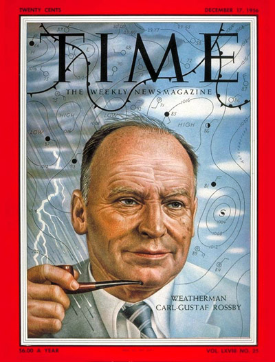
Last Science Tuesday in “Alberta Clippers and Prairie Schooners” I promised to explain why short wavelength weather systems travelled faster than larger storms. I used this science of differential system speeds to explain why I would warn for every Prairie Schooner but maybe not for an Alberta Clipper. My operational mantra was that “small waves moved about half of the 500 mb winds and faster than longer wavelength storms. Really large waves might even retrograde… propagate upstream against the jet stream winds.” We owe the science behind this to figure skaters, conserving spin (angular momentum) and the Einstein of meteorology and a giant of weather prediction, Carl-Gustaf Arvid Rossby (1898-1957). 

In “Revisiting Mountain Ranges and Conserving Spin “, we examined how the jet stream crossing a mountain barrier could create a ridge of high pressure over and upstream from that barrier with a lee trough downstream. Conserving spin in the columns of air flowing over the mountain explained almost everything. In “Lee Cyclogenesis” we described how conserving spin also resulted in very important weather events that formed in the lee of those mountains. Colorado lows can be even more important than Alberta Clippers!

There still remains an important process to explain how to differentiate between these storms and once again, conserving total spin on a rotating sphere is essential. Rossby firmly established this science in 1939. Incredible! He made terrific achievements in understanding the flow of fluids without computers and numerical modelling. We will do the same and you may not be surprised to discover that I will use the deformation zone conceptual model to do so... 

An important secondary circulation develops when the parcels of air follow the wave pattern downstream from the mountains. The total spin of those air parcels must be conserved but that spinning air also impacts the flow and the fluid. I have sketched a weather wave in the accompanying graphic. The wave is also called a planetary wave or even more appropriately, a Rossby wave. These wave patterns are a fact of life in rotating fluids, such as the shallow skin of atmosphere on our rotating Earth. The wave is identical to what one might expect when a strong wind crosses a mountain although I did not include the barrier in the graphic. The dashed grey line can be considered to be the path of the initial strong wind, i.e. blowing from West to East (but that is another story). The air parcels themselves follow the wave pattern that can be seen in the height contours on a weather map – something I explained in an earlier Blog “Mountains and Balancing Spin”. 

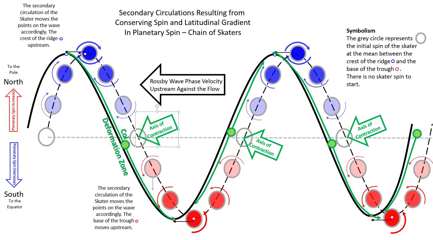
In the graphic I assigned an initial zero spin to an air parcel that is following the wave pattern and deviating from the dashed line. I use the figure skater analogy to simply facilitate the comprehension of the spin of the air parcel.  A skater tracking along the flow over the ridge initially moves toward the pole where cyclonic planetary spin is higher. In order to conserve the total spin, the skater must slow its cyclonic spin down. Since they have no spin to start with, the skater starts to rotate anticyclonically. The sum total of the planetary and skater spin must always remain unchanged. The skater turns toward the equator at the crest of the ridge and starts to gradually shed the anticyclonic spin on the way to the zero spin dashed line. 

As the skater pursues the wave pattern into the trough, they pass through the dashed line of zero spin. Recall that the cyclonic planetary spin always decreases toward the equator. The skater now must experience an increase in cyclonic spin to make up for the loss of planetary spin after crossing the dashed line. At the bottom of the trough, the skater turns to head north again and the cyclonic spin slows down. This process gets repeated again and again and the result is a Rossby wave. 


In this next graphic, I illustrate a chain of skaters distributed along the wave - all with the proper amount of spin required by their distribution on the Earth with respect to the initial dashed grey line. This spin acquired by each skater is required to make up for the northward excesses of cyclonic planetary spin as well as the southward deficits of planetary spin. The cumulative pattern of the spinning skaters required to conserve the total spin is identical to the flow found with a deformation zone! The axis of contraction flow of the deformation zone points directly toward the col and is the wind that moves the original long-dashed  Rossby wave upstream. (see the deformation zone conceptual model below for a refresher). There are only skaters on one side of the deformation zone so that they move the wave pattern in the direction of the axis of contraction flow that created them. This shifted wave is the solid and thicker line in the graphic. The Rossby wave retrogrades against the flow as a result of the spinning skaters interacting with the planetary spin on a rotating Earth. Amazing!

The Blue N in the upper right of this
Deformation Zone Conceptual Model is analogous
to the Blue Spinning Figure Skaters. 
The Red X in the lower right relates to the
Red Spinning Figure Skaters.
I have discussed deformation zones (DZ) many times before in these Art and Science Blogs. See "A Closer Look at Lines in the Sky" among many others.  I repeat the fundamental conceptual model of the Deformation Zone here. The right half of the conceptual model is what I have applied above. 

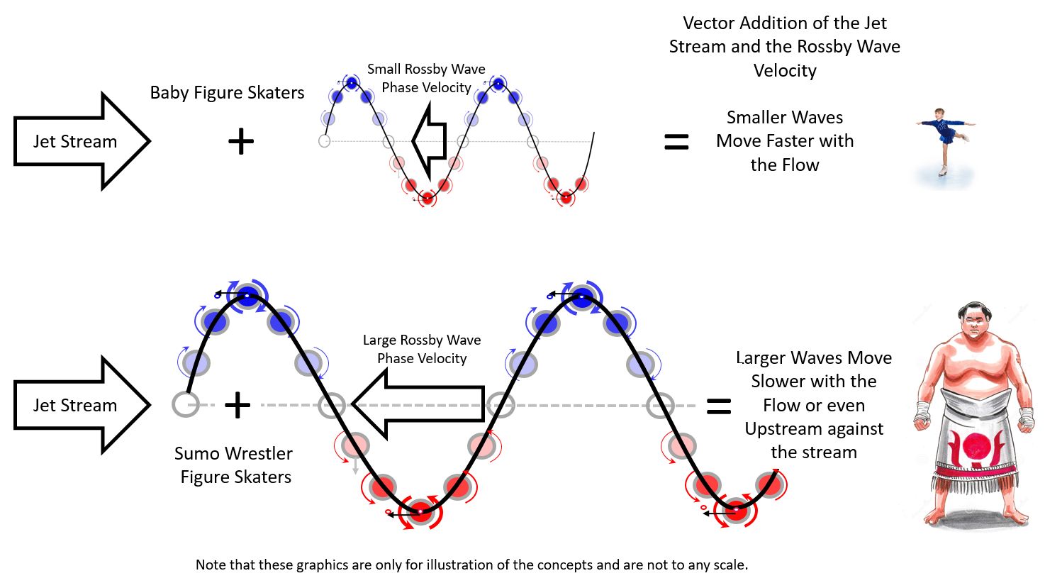
The next graphic illustrates how size is important in determining the intensity of the secondary spinning circulations and thus the speed that the  Rossby wave crests and troughs (Rossby wave phase speed) move upstream.  Imagine the chain of skaters almost holding hands and skating together. The spin of one skater must influence the adjacent skaters both up and downstream - not so simple vector addition. The Rossby wave reacts and moves. While working operationally, I imagined chains of Sumo wrestler skaters versus toddlers just learning to skate. I also wondered if Rossby had these daydream movies playing in his mind. Most of my mental movies occurred on midnight shifts. 

 
Top: Toddler figure skater with short wavelength and small Upstream Rossby Phase Speed
Bottom: Me dressed as a Sumo Wrestler-large wavelength producing
a large Upstream Rossby Phase Speed matching the Jet Stream

The skater size is related to the Rossby wavelength. The secondary circulations required to conserve spin would be correspondingly small for a toddler skater. The Rossby wave phase speed would be equally small and probably much less than the speed of the jet stream that created the initial Rossby wave. The speed of the weather system relative to us living on Earth, is the vector sum of the jet stream winds and the Rossby wave phase speed. The small weather system must move quickly along in the direction of the jet stream but not quite as fast – the 50% rule of thumb that I was taught on MOC (Meteorology Orientation Course) Number 33 way back in 1976. My background was Nuclear Physics and Mathematics and I certainly needed some intensive meteorological training!

A Rossby wave comprised of Sumo wrestler figure skaters also performing together, is an entirely different story. I have performed this Sumo wrestler dance many times to explain these concepts in the weather centre. I am not sure if anyone appreciated where I was headed with those antics but the dance certainly entertained and made my co-workers smile if not laugh . The secondary circulations required to conserve spin for Sumo wrestlers are very large. The Rossby wave phase speed would be equally large and possibly stronger than the jet stream. The larger Rossby wave will certainly be slower moving or even retrograde upstream toward the west.  

And there we have it! Short Rossby wavelength systems are likely to be carried with the jet stream. As the wavelength of the Rossby wave gradually increases, the weather moves ever slower and may even start to head upstream. And this is why I warned for the longer wavelength Prairie Schooners and possibly not for the shorter wavelength Alberta Clippers. 

My friend, retired Professor Ed Lozowski of the University of Alberta, has read this Blog. He suggested another interesting analogy of the long wavelength pattern moving upstream in the flow to be similar to a huge salmon whereas the smaller waves get flushed with the flow like minnows. Ed made several thoughtful, accurate suggestions and refinements and I am indebted to his breadth of knowledge and generosity. I own any and all errors that might remain. 

There are many ways to examine nature and to try to understand the science. Rossby liked the rigourous mathematics of differential equations but the results must be physically the same whatever your favourite analogy might be. Rossby was really quite incredible.

Warmest regards and keep your paddle in the water,

Phil the Forecaster Chadwick