Science Tuesday - Smelling the Roses

#2623 "Red Cedar Shelter 12x10 panel

This is the weather equivalent of stopping to smell the roses.  I posted a painting of this red cedar in #2623 "Red Cedar Shelter" just yesterday and lee cyclogenesis has provided a beautiful April snowfall. This event summarizes the science of the past four months and we only need to enjoy. We do not need to investigate the terminal velocity of snowflakes today. 

We started in January with "Know the Wind". If you know the wind, you will learn the weather. Each week we added to the science culminating with Rossby waves and "The Weather Race of Alberta Clippers and Prairie Schooners" last Tuesday. 

Today we relax and enjoy the snow and the science that we have embraced. Science, art and the meaning of life are all entwined together... 

Warmest regards and keep your paddle in the water,

Phil the Forecaster Chadwick

The Weather Race of Alberta Clippers and Prairie Schooners...

#2609 "Jim Day Rapids Point" 16x20
Lots of snow from a slow moving Prairie Schooner

The laws of physics make perfect sense even if we might not fully understand them. Operationally, in the weather forecast office, one cannot afford the time to go back to first principles and savour the science. The forecast needs to go out on time if not early. A late forecast becomes just an observation and not much help in giving people the opportunity to plan for life, safety and their economy. 

There were many times on shift when something unexpected appeared in the data and I wondered why! What does that pattern really mean? Nature is always right. I often did not have the luxury of time to investigate those facts. Retirement means I have more hours now… and that also explains the motivation behind these blogs… and sharing the beauty of nature, science and art. They can all really be the same. 

Last Science Tuesday in “Alberta Clippers and Prairie Schooners” I promised to explain why short wavelength weather systems travelled faster than larger storms. I used this science of differential system speeds to explain why I would warn for every Prairie Schooner but maybe not for an Alberta Clipper. My operational mantra was that “small waves moved about half of the 500 mb winds and faster than longer wavelength storms. Really large waves might even retrograde… propagate upstream against the jet stream winds.” We owe the science behind this to figure skaters, conserving spin (angular momentum) and the Einstein of meteorology and a giant of weather prediction, Carl-Gustaf Arvid Rossby (1898-1957). 

In “Revisiting Mountain Ranges and Conserving Spin “, we examined how the jet stream crossing a mountain barrier could create a ridge of high pressure over and upstream from that barrier with a lee trough downstream. Conserving spin in the columns of air flowing over the mountain explained almost everything. In “Lee Cyclogenesis” we described how conserving spin also resulted in very important weather events that formed in the lee of those mountains. Colorado lows can be even more important than Alberta Clippers!

There still remains an important process to explain how to differentiate between these storms and once again, conserving total spin on a rotating sphere is essential. Rossby firmly established this science in 1939. Incredible! He made terrific achievements in understanding the flow of fluids without computers and numerical modelling. We will do the same and you may not be surprised to discover that I will use the deformation zone conceptual model to do so... 

An important secondary circulation develops when the parcels of air follow the wave pattern downstream from the mountains. The total spin of those air parcels must be conserved but that spinning air also impacts the flow and the fluid. I have sketched a weather wave in the accompanying graphic. The wave is also called a planetary wave or even more appropriately, a Rossby wave. These wave patterns are a fact of life in rotating fluids, such as the shallow skin of atmosphere on our rotating Earth. The wave is identical to what one might expect when a strong wind crosses a mountain although I did not include the barrier in the graphic. The dashed grey line can be considered to be the path of the initial strong wind, i.e. blowing from West to East (but that is another story). The air parcels themselves follow the wave pattern that can be seen in the height contours on a weather map – something I explained in an earlier Blog “Mountains and Balancing Spin”. 

In the graphic I assigned an initial zero spin to an air parcel that is following the wave pattern and deviating from the dashed line. I use the figure skater analogy to simply facilitate the comprehension of the spin of the air parcel.  A skater tracking along the flow over the ridge initially moves toward the pole where cyclonic planetary spin is higher. In order to conserve the total spin, the skater must slow its cyclonic spin down. Since they have no spin to start with, the skater starts to rotate anticyclonically. The sum total of the planetary and skater spin must always remain unchanged. The skater turns toward the equator at the crest of the ridge and starts to gradually shed the anticyclonic spin on the way to the zero spin dashed line. 

As the skater pursues the wave pattern into the trough, they pass through the dashed line of zero spin. Recall that the cyclonic planetary spin always decreases toward the equator. The skater now must experience an increase in cyclonic spin to make up for the loss of planetary spin after crossing the dashed line. At the bottom of the trough, the skater turns to head north again and the cyclonic spin slows down. This process gets repeated again and again and the result is a Rossby wave. 

In this next graphic, I illustrate a chain of skaters distributed along the wave - all with the proper amount of spin required by their distribution on the Earth with respect to the initial dashed grey line. This spin acquired by each skater is required to make up for the northward excesses of cyclonic planetary spin as well as the southward deficits of planetary spin. The cumulative pattern of the spinning skaters required to conserve the total spin is identical to the flow found with a deformation zone! The axis of contraction flow of the deformation zone points directly toward the col and is the wind that moves the original long-dashed  Rossby wave upstream. (see the deformation zone conceptual model below for a refresher). There are only skaters on one side of the deformation zone so that they move the wave pattern in the direction of the axis of contraction flow that created them. This shifted wave is the solid and thicker line in the graphic. The Rossby wave retrogrades against the flow as a result of the spinning skaters interacting with the planetary spin on a rotating Earth. Amazing!

The Blue N in the upper right of this
Deformation Zone Conceptual Model is analogous
to the Blue Spinning Figure Skaters. 
The Red X in the lower right relates to the
Red Spinning Figure Skaters.

I have discussed deformation zones (DZ) many times before in these Art and Science Blogs. See "A Closer Look at Lines in the Sky" among many others.  I repeat the fundamental conceptual model of the Deformation Zone here. The right half of the conceptual model is what I have applied above. 

The next graphic illustrates how size is important in determining the intensity of the secondary spinning circulations and thus the speed that the  Rossby wave crests and troughs (Rossby wave phase speed) move upstream.  Imagine the chain of skaters almost holding hands and skating together. The spin of one skater must influence the adjacent skaters both up and downstream - not so simple vector addition. The Rossby wave reacts and moves. While working operationally, I imagined chains of Sumo wrestler skaters versus toddlers just learning to skate. I also wondered if Rossby had these daydream movies playing in his mind. Most of my mental movies occurred on midnight shifts. 

 

Top: Toddler figure skater with short wavelength and small Upstream Rossby Phase Speed
Bottom: Me dressed as a Sumo Wrestler-large wavelength producing
a large Upstream Rossby Phase Speed matching the Jet Stream

The skater size is related to the Rossby wavelength. The secondary circulations required to conserve spin would be correspondingly small for a toddler skater. The Rossby wave phase speed would be equally small and probably much less than the speed of the jet stream that created the initial Rossby wave. The speed of the weather system relative to us living on Earth, is the vector sum of the jet stream winds and the Rossby wave phase speed. The small weather system must move quickly along in the direction of the jet stream but not quite as fast – the 50% rule of thumb that I was taught on MOC (Meteorology Orientation Course) Number 33 way back in 1976. My background was Nuclear Physics and Mathematics and I certainly needed some intensive meteorological training!

A Rossby wave comprised of Sumo wrestler figure skaters also performing together, is an entirely different story. I have performed this Sumo wrestler dance many times to explain these concepts in the weather centre. I am not sure if anyone appreciated where I was headed with those antics but the dance certainly entertained and made my co-workers smile if not laugh . The secondary circulations required to conserve spin for Sumo wrestlers are very large. The Rossby wave phase speed would be equally large and possibly stronger than the jet stream. The larger Rossby wave will certainly be slower moving or even retrograde upstream toward the west.  

And there we have it! Short Rossby wavelength systems are likely to be carried with the jet stream. As the wavelength of the Rossby wave gradually increases, the weather moves ever slower and may even start to head upstream. And this is why I warned for the longer wavelength Prairie Schooners and possibly not for the shorter wavelength Alberta Clippers. 

My friend, retired Professor Ed Lozowski of the University of Alberta, has read this Blog. He suggested another interesting analogy of the long wavelength pattern moving upstream in the flow to be similar to a huge salmon whereas the smaller waves get flushed with the flow like minnows. Ed made several thoughtful, accurate suggestions and refinements and I am indebted to his breadth of knowledge and generosity. I own any and all errors that might remain. 

There are many ways to examine nature and to try to understand the science. Rossby liked the rigourous mathematics of differential equations but the results must be physically the same whatever your favourite analogy might be. Rossby was really quite incredible.

Warmest regards and keep your paddle in the water,

Phil the Forecaster Chadwick

Alberta Clippers and Prairie Schooners

#2611 "Winter Tree Tunnel" 
20x16 inches oils gallery wrapped
40 centimetres of Singleton snow
after a Prairie Schooner

In the past few Science Stories, we have established how lee cyclogenesis is linked to conserving the spin of a figure skater. We briefly investigated how the temperatures of the equatorial Pacific Ocean influences the location of the jet stream and why there were more Alberta Clippers in a LaNiña year like 2022.  These storms are an essential part of the global balance. Weather results from an imbalance in one or all of the basic components of the energy cycle: heat, cold, water, electrical charge and there are certainly other forms of energy to juggle and try to distribute judiciously.

In advance of a low pressure area (a storm), warm and moist air is moved northward. In the wake of that low, cold and relatively dry air is moved southward. The pressure pattern that results is really a wave in the atmosphere … the downstream ridge is separated from the upstream trough by the storm and the next upstream ridge. Together the atmospheric wave which is the storm attempts to keep the earth in balance. The wavelength is from one ridge to the next. 

The impact of an atmospheric wave is related to its size - just like waves on the ocean. Winter weather can also have more impact than summer. Although severe summer convection can be extremely exciting and dangerous, the impacts on society and the economy are often more important with the winds, temperature and precipitation of “ordinary”, everyday winter weather. Such is the case with Alberta Clippers and this is where we have been headed all along. 

Genesis Stage of an Alberta Clipper

The impacts of Alberta clippers also vary with the size of the storm. The scale of an individual clipper varies with the strength of the jet stream crossing the Rockies, the size and intensity of the lee cyclogenesis and the temperature contrast across the frontal zone. There are other factors for sure but let’s keep this simple. We will even start with some history. 

The name “Alberta Clipper” was coined in the late 1960s by Rheinhart Harms, a meteorologist at the U.S. National Weather Service Office in Milwaukee, Wisconsin. Rheinhart witnessed the rapid speed of these snow storms as they crossed the Prairies. I undoubtedly heard the term when I entered the world of meteorology in the 1970s. It would take until the 1990s for that phrase to enter the scientific literature.

Alberta clippers are frequent winter forecast challenges and can occur every few days in rapid succession just as they did in February 2022. The first clue is to witness the jet stream crossing the Alberta Rockies nearly perpendicularly. A chinook arch is typical when those westerly winds charge down the lee slopes to dig the lee the trough. The chinook brings relatively warm weather approaching 10 °C even in the middle of winter. Lee cyclogenesis follows as the energy of the jet stream and the “figure skater” is transformed into a low pressure area and wave that then ripples along with the jet stream.

The clippers approach fast. Snowfall amounts with these systems tend to be small with only 3 to 8 cm being typical. The lack of moisture and short duration keep the accumulation well below the warning impact threshold of 15 cm per 12 hours. 

The wind and the wind chills can be more important for the typical clipper. Temperatures typically drop 15 to 20 Celsius degrees in just a few hours behind the clipper cold front. Blowing and drifting of even the small amounts of snow can make travel treacherous in whiteout conditions. These situations can approach warning criteria. 

Alberta Clipper crossing the Great Lakes

As the clipper cross the Great Lakes, the dynamics of the storm can change. When combined, the five great lakes represent a huge source of heat and moisture as well as lower friction. The inland seas also provide the opportunity for the generation of snowsqualls when those strong, cold Arctic winds blow over the open waters of the lakes. Snowsqualls bring significant snow accumulations onshore as well as extensive whiteout conditions  – that is another story that we call lake-effect snow. Suffice it to say that Alberta Clippers can take on a different and potentially dangerous character when they cross the Great Lakes to affect Ontario, Quebec and the north-eastern United States. 

I spent a large part of my meteorological career very concerned about how Alberta Clippers would influence my forecast regions. In the early 1990’s I was looking for a simple way to differentiate between the impact and the threat of each of these storms emerging every few days from the Rockies of Alberta. The larger the storm, the more probable that warning criteria would be breached and this could all be summarized by the speed of the clipper. 

I started using the phrase “Prairie Schooner” to describe these larger storms that would produce warning criteria weather. Clippers were built for speed but for me, schooners delivered the goods! Often, clippers were rebuilt into schooners as they crossed the “Great Lakes Aggregate” as we described the combined effects of those inland seas. As I recall, clippers would sail along at about 30 knots but schooners moved slower at only 20 knots. I kept careful histories of the track and speed of these storms emerging from Alberta. Any clipper that was slowing down to 20 knots was doing so for good meteorological reasons and I would get ready to hoist the warnings and rebrand that weather event as a Prairie Schooner. 

The science of the storm was all embedded in the speed of the system. Temperature contrast, precipitation rate and duration, latent heat … there is a long list that goes into determining the size of the storm. And size determines the wavelength which governs the speed. 

In 2005 my meteorological career took me to COMET (https://www.comet.ucar.edu/) in Boulder, Colorado. I recall that the acronym stands for something like “Cooperative Program for Operational Meteorology, Education and Training” but no one in that office even uses that anymore. Some of these Blogs were turned into Training Modules by the professional team of instructional designers, scientists, graphic artists, multimedia developers, and information technologists of COMET, UCAR and NOAA’s National Weather Service. After seven years in Boulder, I gradually retired during the course of the last decade – but not totally. 

The distinction between Alberta Clippers and Prairie Schooners has possibly been forgotten or perhaps I did not explain the concepts well enough. This Blog was intended to mend the sails on that ship – the concepts are simple, effective and fun at the same time. 

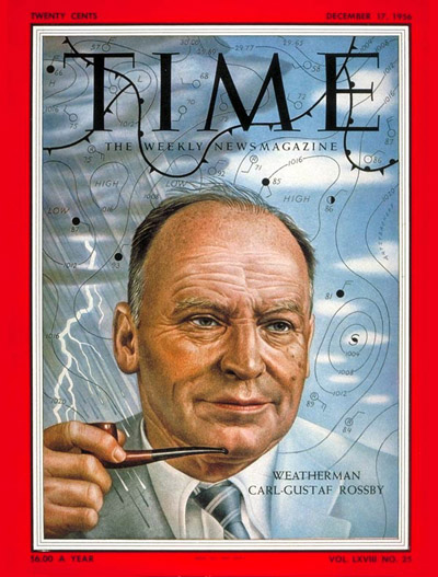
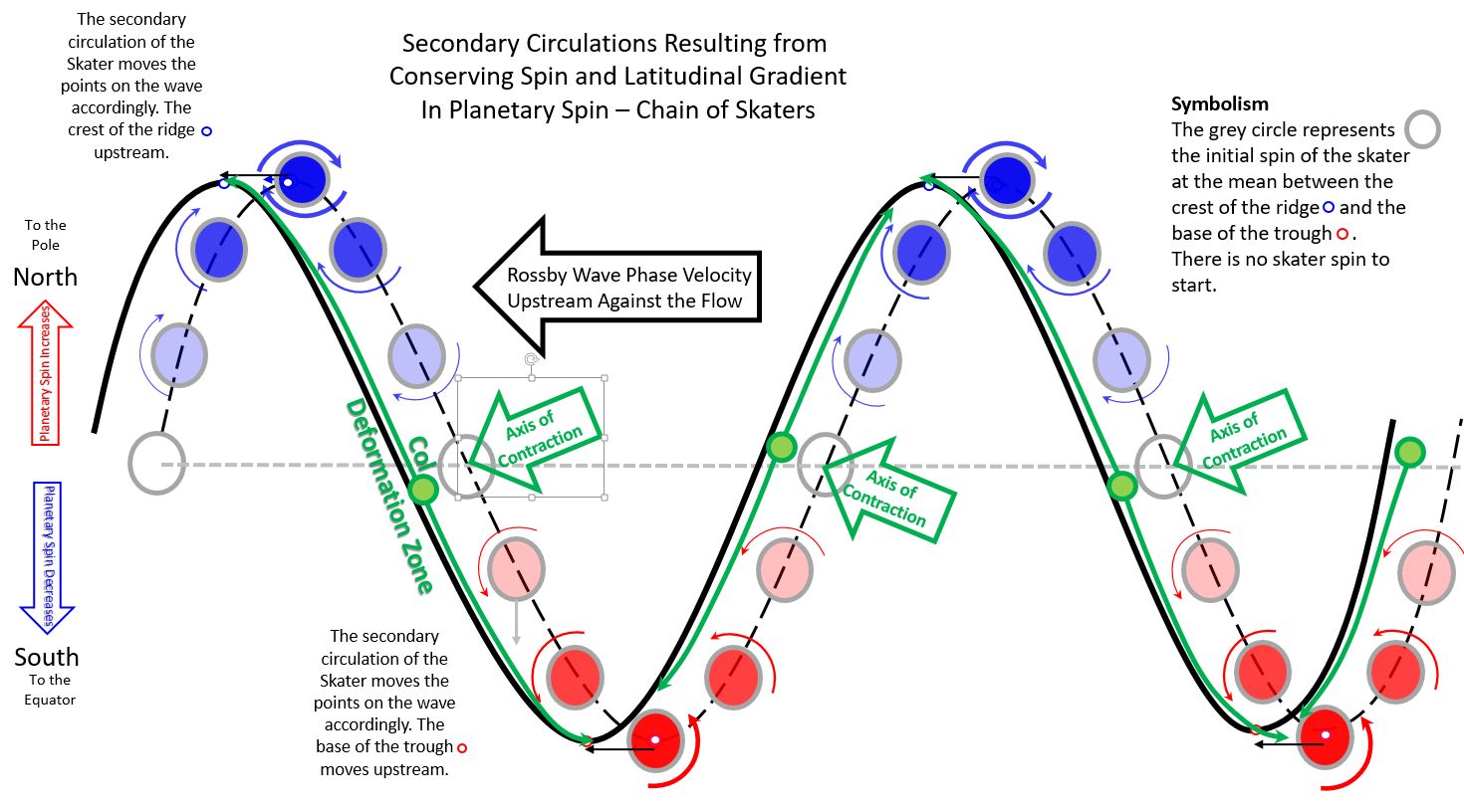
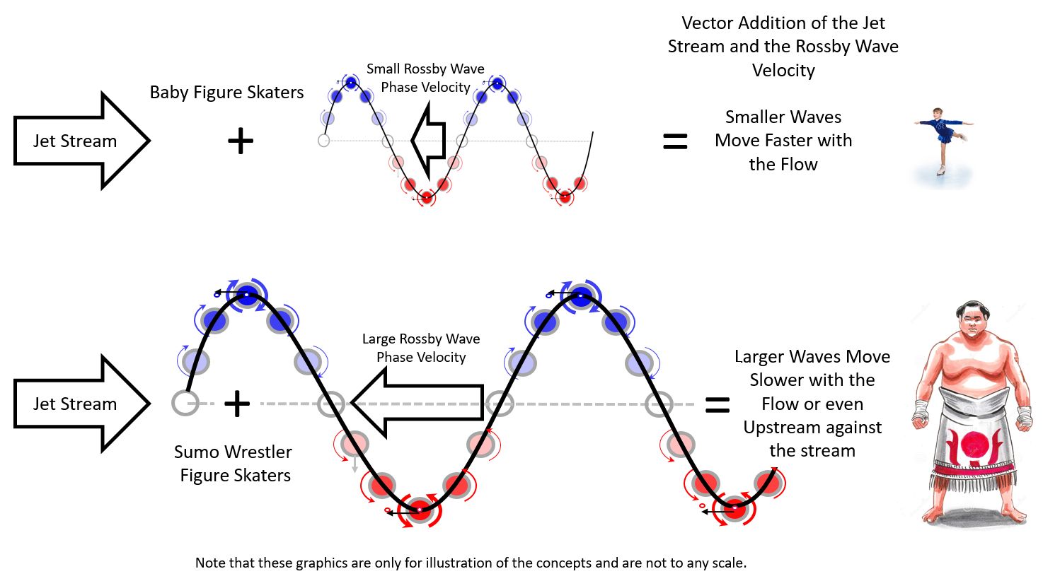
Next week we will explain why small Alberta Clippers are faster than Prairie Schooners. It will all make sense with the assistance of meteorologist Carl-Gustaf Arvid Rossby and our friend the figure skater as we conserve spin also known as angular momentum. 

Warmest regards and keep your paddle in the water, be safe,

Phil the Forecaster Chadwick